1. Short history

In 1972, Robert Rescorla and Allan Wagner developed a formal theory of associative learning, the process through which multiple stimuli are associated with one-another. The most widely used example (Fig. 1) of associative learning comes straight from Psychology 101–Pavlov’s dog.

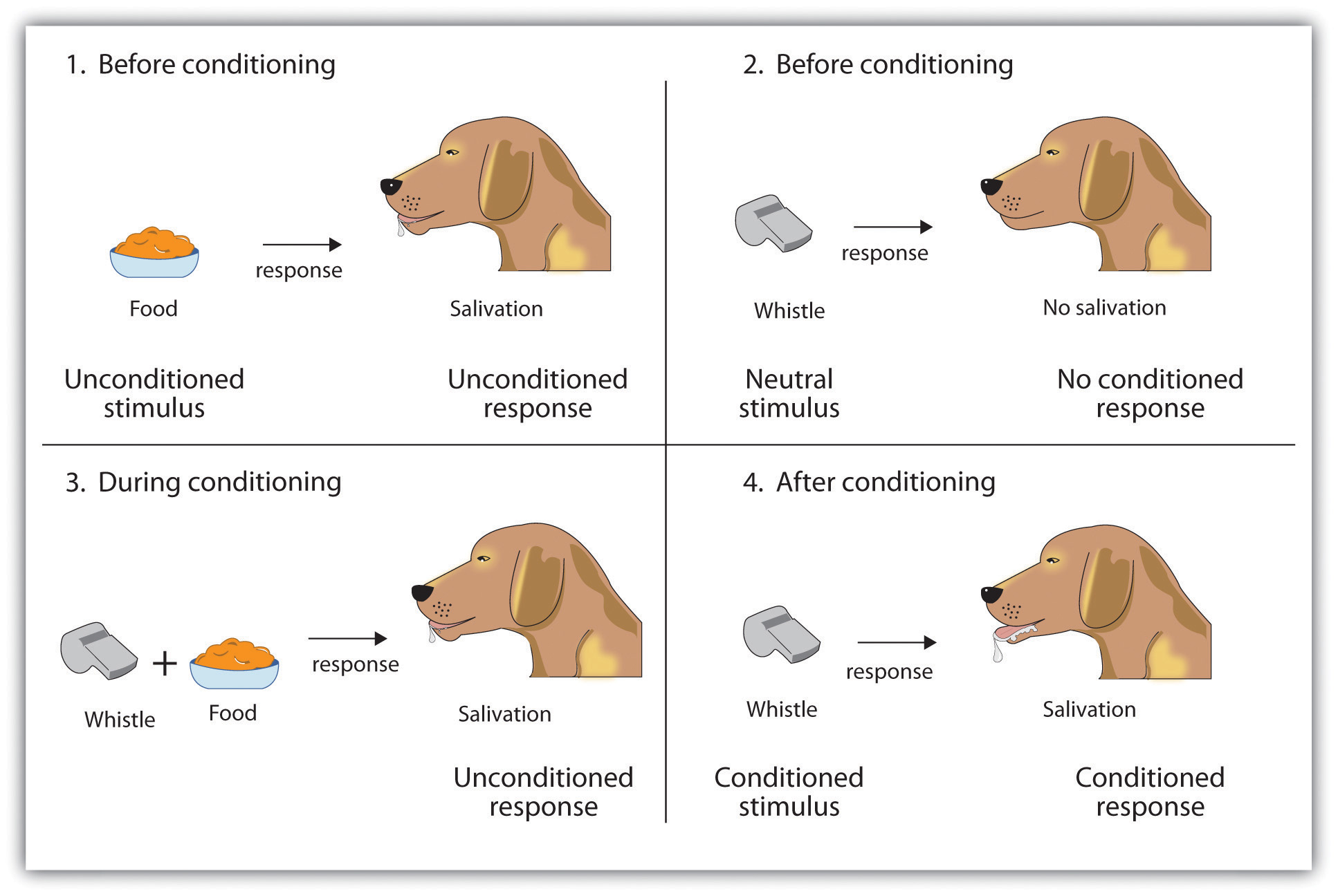
Figure 1

The idea is simple, and it’s something that we experience quite often in everyday life. In the same way that Pavlov’s dog begins to drool after hearing a bell, certain cognitive and/or biological processes are triggered when we are exposed to stimuli that we have been exposed to in the past. But how can this learning process be modeled? That is to say, what sort of equation can we use to describe how an agent learns to associate multiple stimuli? To answer these questions, Rescorla and Wagner developed what is now know as the Rescorla-Wagner updating rule:

\[\Delta V_{A} = \alpha_{A} \beta_{1} (\lambda_{1} - V_{AX})\]

\[\Delta V_{X} = \alpha_{X} \beta_{1} (\lambda_{1} - V_{AX})\]

First off, note that the original Rescorla-Wagner rule was developed to explain compound stimuli (e.g. presentation of a bell and light, followed by food). Here, \(\Delta V_{A}\) is the change in associative strength between stimulus \(A\) (e.g. the bell) and the response (e.g. food). \(\Delta V_{X}\) has the same interpretation, but refers to stimulus \(X\) (e.g. the light).

\(0 \leq \beta_{1} \leq 1\) is a free parameter (i.e. we estimate it from the data) referred to as the learning rate. The learning rate controls how quickly updating takes place, where values near 0 and 1 reflect sluggish and rapid learning, respectively. Above, the learning rate is shared across stimuli.

\(0 \leq \alpha_{A} \leq 1\) is a free parameter which is determined by the salience of stimulus \(A\), and \(0 \leq \alpha_{X} \leq 1\) for stimulus \(X\). Unlike the learning rate, which is shared across stimuli, the salience parameter is specific to each stimulus. Put simply, this just means that learning can occur at different rates depending on the type of stimulus (e.g. I may associate a light with food more quickly than a tone).

\(\lambda_{1}\) is described as “the asymptote of associative strength”. This is the upper-limit on how strong the association strength can be. In this way, \(\lambda_{1}\) reflects the value being updated toward by the learning rate (\(\beta\)) and stimulus salience (\(\alpha\)).

Lastly, \(V_{AX}\) is the total associative strength of the compound stimulus \(AX\). Rescorla and Wagner assume that this is a simple sum of both stimuli strengths:

\[V_{AX} = V_{A} + V_{X}\]

Interpretation of this model is actually quite simple–we update associative strength (\(V_{*}\)) for each stimulus by taking steps (\(\alpha \beta\)) toward the difference between the asymptote of learning (\(\lambda_{1}\)) and the current associative strength of the compund stimulus (\(V_{AX}\)). By continually exposing an agent to a tone or bell paired with a reward (or punishment), the agent learns the associative strength of the conditioned and unconditioned stimuli.

While the original Rescorla-Wagner model was successful for explaining associative learning for classical conditioning paradigms, what of operant conditioning? What if we are interested in how people learn to make decisions? In most current research, we are not interested in knowing how people learn to associate lights or tones with some reward. Instead, we would like a model that can describe how people learn to select the best choice among multiple choices. This model would need to explain how people assign values to multiple options as well as how they decide which option to choose. In statistical terms, we want to know how people solve the multi-armed bandit problem. In the following section, we will begin to solve this problem.

2. Current Implementations

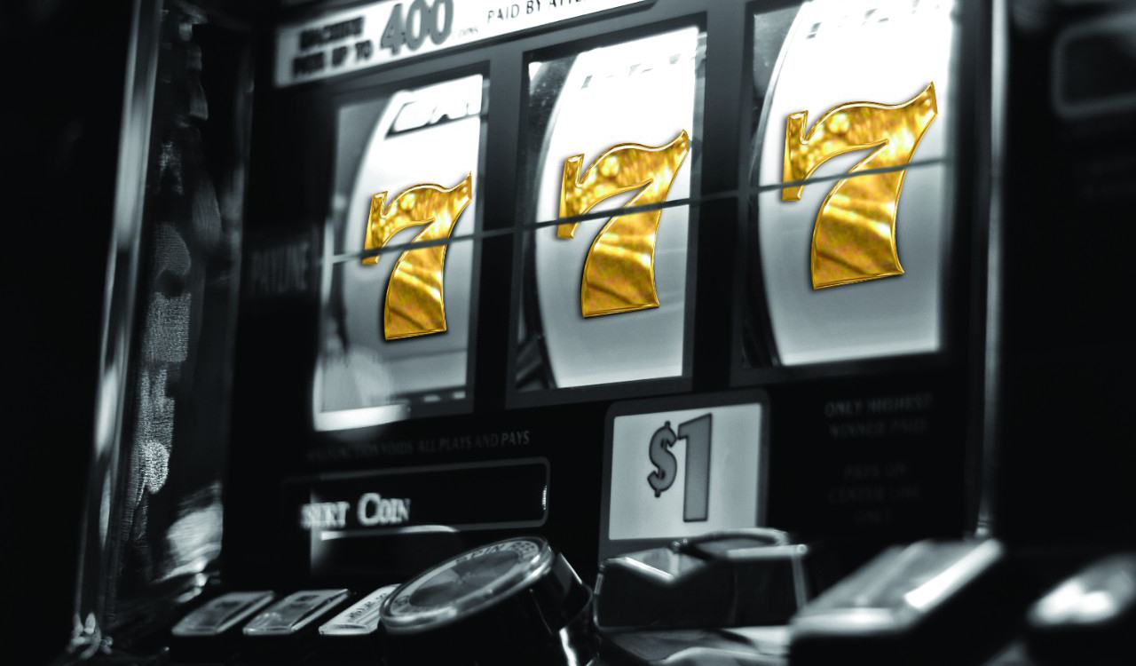
Figure 1

As a motivating example, we will explore the simple problem of learning the probability that a slot machine will payoff (i.e. that you will win any amount after pulling the lever). To do so, the above equations only need minor modifications. Additionally, we will change the terminology–instead of learning an associative strength, we will now be learning the probability of a winning outcome. To start, we take the first equation above and write it for a single stimulus \(V\), but exchange \(V\) with the probability of observing a win:

\[\Delta Pr(win) = \alpha \beta (\lambda - Pr(win))\]

Because \(\Delta Pr(win) = Pr(win)_{t+1} - Pr(win)_{t}\) (where \(t\) is the current trial), we can re-write the above equation into an iterative form:

\[Pr(win)_{t+1} = Pr(win)_{t} + \alpha \beta (\lambda_{t} - Pr(win)_{t})\]

Since we are using this model to explain how people learn the probability of a binary outcome, \(\lambda_{t} \in [0, 1]\) now represents the outcome of slot machine roll on trial \(t\). Now, we drop the \(\alpha\) parameter to simplify the model further. Because we have a single choice option, estimating both \(\alpha\) and \(\beta\) would lead to an unidentifiable model. This is because as either one increases, the other can decrease and lead to the same exact predictions. Even with multiple choice options, this problem is still apparent. In current applications of the Rescorla-Wagner rule, we do not include a “salience” parameter. Now, we have:

\[Pr(win)_{t+1} = Pr(win)_{t} + \beta (\lambda_{t} - Pr(win)_{t})\]

The model is now much easier to interpret. The term \((\lambda_{t} - Pr(win)_{t})\) can be thought of as the prediction error–the difference between the actual value \(\lambda_{t}\) revealed after the choice was made and the expected value of the choice \(Pr(win)_{t}\) for that trial. \(\beta\) (the learning rate) then updates the current expectation \(Pr(win)_{t}\) in the direction of the prediction error \((\lambda_{t} - Pr(win)_{t})\).

3. R Example

To see the Rescorla-Wagner rule in action, let’s generate some fake data using the binomial distribution and try to estimate the rate parameter using various different values for the learning rate.

# For pretty images
library(ggplot2)

# Number of 'trials'
num_trials <- 100

# The win rate is 0.7
payoff <- rbinom(n = num_trials, size = 1, prob = 0.7)

# Function that iterates the Rescorla-Wagner rule 
rw_update <- function(lambda, beta, init) {
  # To store expected value for each trial
  Pr_win <- vector(length=length(lambda))
  # Set initial value
  Pr_win[1] <- init
  for (t in 1:(length(lambda)-1)) {
    Pr_win[t+1] <- Pr_win[t] + beta * (lambda[t] - Pr_win[t])
  }
  return(Pr_win)
}

# With initial expectation = 0, try different learning rates
beta_05 <- rw_update(lambda = payoff, beta = 0.05, init = 0)
beta_25 <- rw_update(lambda = payoff, beta = 0.25, init = 0)
beta_50 <- rw_update(lambda = payoff, beta = 0.50, init = 0)
beta_75 <- rw_update(lambda = payoff, beta = 0.75, init = 0)
beta_95 <- rw_update(lambda = payoff, beta = 0.95, init = 0)

# Store in data.frame for plotting
all_data <- stack(data.frame(beta_05 = beta_05,
                             beta_25 = beta_25,
                             beta_50 = beta_50,
                             beta_75 = beta_75,
                             beta_95 = beta_95))
# Add trial 
all_data[["trial"]] <- rep(1:num_trials, 5)
names(all_data)[2]  <- "Beta"

# Plot results
p <- ggplot(all_data, aes(x = trial, y = values, color = Beta)) + 
  geom_line() + 
  geom_hline(yintercept = 0.7, colour="black", linetype = "longdash") + 
  ggtitle("Expected Probability of Winning Outcome") + 
  xlab("Trial Number") + 
  ylab("Expected Pr(win)")  
p

It is easy to see that the higher learning rates (i.e. > 0.05) are jumping around the true win rate (0.7, dashed line) quite a bit, whereas setting \(\beta = 0.05\) allows for a more stable estimate. Let’s try again with learning rates closer to 0.05.

# Learning rates closer to 0.05
beta_01 <- rw_update(lambda = payoff, beta = 0.01, init = 0)
beta_03 <- rw_update(lambda = payoff, beta = 0.03, init = 0)
beta_05 <- rw_update(lambda = payoff, beta = 0.05, init = 0)
beta_07 <- rw_update(lambda = payoff, beta = 0.07, init = 0)
beta_09 <- rw_update(lambda = payoff, beta = 0.09, init = 0)

# Store in data.frame for plotting
all_data <- stack(data.frame(beta_01 = beta_01,
                             beta_03 = beta_03,
                             beta_05 = beta_05,
                             beta_07 = beta_07,
                             beta_09 = beta_09))
# Add trial 
all_data[["trial"]] <- rep(1:num_trials, 5)
names(all_data)[2]  <- "Beta"

# Plot results
p2 <- ggplot(all_data, aes(x = trial, y = values, color = Beta)) +
  geom_line() + 
  geom_hline(yintercept = 0.7, colour="black", linetype = "longdash") + 
  ggtitle("Expected Probability of Winning Outcome") + 
  xlab("Trial Number") + 
  ylab("Expected Pr(win)")
p2

These results look a bit better. However, it is apparent that setting \(\beta\) too low is making the updating very sluggish. If we run more trials, however, we should see the expectation converge.

# Number of 'trials'
num_trials <- 500

# The win rate is 0.7
payoff <- rbinom(n = num_trials, size = 1, prob = 0.7)

# Learning rates closer to 0.05
beta_01 <- rw_update(lambda = payoff, beta = 0.01, init = 0)
beta_03 <- rw_update(lambda = payoff, beta = 0.03, init = 0)
beta_05 <- rw_update(lambda = payoff, beta = 0.05, init = 0)
beta_07 <- rw_update(lambda = payoff, beta = 0.07, init = 0)
beta_09 <- rw_update(lambda = payoff, beta = 0.09, init = 0)

# Store in data.frame for plotting
all_data <- stack(data.frame(beta_01 = beta_01,
                             beta_03 = beta_03,
                             beta_05 = beta_05,
                             beta_07 = beta_07,
                             beta_09 = beta_09))
# Add trial 
all_data[["trial"]] <- rep(1:num_trials, 5)
names(all_data)[2]  <- "Beta"

# Plot results
p2 <- ggplot(all_data, aes(x = trial, y = values, color = Beta)) +
  geom_line() + 
  geom_hline(yintercept = 0.7, colour="black", linetype = "longdash") + 
  ggtitle("Expected Probability of Winning Outcome") + 
  xlab("Trial Number") + 
  ylab("Expected Pr(win)")
p2

Over 500 trials, the expected value for the win rate converges to the true win rate, 70%.

4. Summary

In this post, we reviewed the original Rescorla-Wagner updating rule (a.k.a. the Delta Rule) and explored its contemporary instantiation. I have shown that the Delta Rule can be used to estimate the win rate of a slot machine on a trial-by-trial basis. While this example may first appear trivial (e.g. why not just take the average of all past outcomes?), we will explore more practical usages in later posts. For now, try playing with the above code yourself! If you want a slightly more challenging problem, try finding the solution to the following question:

• How should you change the learning rate so that the expected win rate is always the average of all past outcomes?

• Hint –> With some simple algebra, the Delta Rule can be re-written as follows:

\[Pr(win)_{t+1} = (1 - \beta) \cdot Pr(win)_{t} + \beta \cdot \lambda_{t}\]

Happy solving! See the answer in the next post.