Bayesian Design Optimization: An Application to Item Reduction in Scale Development Research

Goals
Survey-based measures are used throughout the social, behavioral, and health sciences–but how are they developed? And how do we know they measure the constructs they are meant to measure? The answers to these questions lie somewhere in the field of “scale development”, a research area within psychometrics more broadly wherein researchers develop and test theories on how to create reliable, valid survey-based measures.
In this post, we will dive deep into a particular set of psychometric methods; namely, those used to reduce down a large pool of survey items to a smaller, more manageable set while retaining the most information possible. In doing so, we will touch on many topics including reliability, information theory, Bayes Factors, and more. My hope is that you will leave this blog with a better understanding of what survey items are from a statistical perspective, in addition to understanding some pitfalls of traditional methods used to develop surveys.
This post is will be broken into two parts. Part 1 will lay out competing strategies for measuring how informative an item or set of items is. Part 2 will build upon Part 1, illustrating how to select a subset of items given various item informativeness measures.
Part 1: Understanding your items
A classical view
Historically, Cronbach’s \(\alpha\)–often referred to as a measure of internal consistency–has played a large role in helping researchers understand how informative a set of items is. Before we dive into why, let’s take a look at how Cronbach’s \(\alpha\) is defined:
\[ \begin{equation} \alpha = \frac{N}{N - 1} \left(1 - \frac{\sum_{i=1}^N \sigma_i^2}{\sigma^2_\text{total}}\right) \tag{1} \end{equation} \]
Here, \(\sigma_i^2\) is the variance of the \(i\)th item, and \(\sigma^2_\text{total}\) is the variance across total test scores. In our case, the total test score for each person is just the sum score across items for each person. To better understand the math, take a look at the R code below that estimates \(\alpha\) given a small set of respondents:
# Pseudo-data: columns = items, rows = people
data <- matrix(
  c(
    1, 2, 3, 4,
    2, 2, 3, 5,
    1, 3, 4, 4,
    2, 3, 5, 5
  ),
  nrow = 4,
  byrow = TRUE
)

# Number of items
N <- ncol(data)

# sigma_i = variance of item i across people
item_variances <- apply(data, 2, var)

# score for each person
total_scores <- rowSums(data)

# sigma_total = variance of total scores across people
total_variance <- var(total_scores)

# Cronbach's alpha
alpha <- (N / (N - 1)) * (1 - sum(item_variances) / total_variance)
Here, \(\alpha =\) 0.73. Given a few assumptions, we can think of \(\alpha\) as the average item-level correlation with the underlying “true score” of the latent trait our items measure. Higher \(\alpha\) indicates higher correlation, meaning that the score we derive for each person is closer to the true score we aim to measure. We cover how reliability affects true score estimation in depth in a pevious post, but the main take-away here is that a set of items with higher reliability equates to a survey that is more informative with respect to the latent trait of interest. If reliability were perfect for a given set of items (i.e. \(\alpha = 1\)), there would exist no other items that could offer further information on the underlying latent trait.
However, usage of \(\alpha\) assumes many things about our scale that may not be true in practice, including but not limited to the following:
- our scale is unidimensional,
- items are tau-equivalent (i.e. all items have the same true-score variance and load equally onto the latent trait),
- item-level errors are uncorrelated (i.e. given the latent trait and item parameters, item responses are independent), and
- relationships between item scores and true scores is linear
Such restrictive assumptions impact the type of survey that one can use \(\alpha\) on for item selection, and in fact they encourage researchers to make simplifying assumptions about constructs that may deviate from the substantive theory motivating scale development in the first place.
An Item Response Theory view
Item-response theory (IRT) provides a more generative framework through which we can view survey response behavior, which allows for us to build models that more clearly map to our substantive theory of the underlying construct(s) we aim to measure (see our pevious post for a bit more on how). Alongside the added theoretical flexibility, IRT introduces new ways to conceptualize reliability–not as a single global metric, but as something that can vary locally depending on the trait level being measured. Put simply, IRT captures the fact that different items provide different levels of information across different people, making it possible to customize surveys to more precisely measure traits in populations of interest.
The conceptual shift from reliability to information
The shift from classical approaches to IRT also opens the door to more sophisticated approaches to assess item informativeness. Historically, the concept of item information has been used. Item information is the Fisher Information of an item. Whereas Cronbach’s \(\alpha\) reflects the reliability of a scale by assessing how well the items collectively covary with the assumed latent construct, Fisher information is a more granular measure that evaluates measurement precision for individual items across specific regions of the latent parameter space (\(\theta\)).
It is easier to understand the concept of item information by visualizing item information curves across the latent trait. For example, let’s consider a simple 2-parameter logistic (2PL) IRT model. This model specifies the probability that an individual with a latent trait level \(\theta\) answers an item \(i\) with two response options as follows:
\[ \begin{equation} p_{i}(y_i = 1 \mid \theta) = \frac{1}{1 + e^{-a_i (\theta - b_i)}} \tag{2} \end{equation} \]
where:
- \(a_i\) is the discrimination parameter, capturing how sharply the item differentiates between individuals with different levels of \(\theta\), and
- \(b_i\) is the difficulty parameter, indicating the level of \(\theta\) at which the item has a 50% chance of being answered with a 0 versus 1 response (i.e. disagree vs agree, etc.),
The item information curve (i.e. the Fisher information curve, we will use the terms interchangeably) for the 2PL model is then:
\[ \begin{equation} I_{i}(\theta) = a^2 p_{i}(\theta)(1-p_{i}(\theta)) \tag{3} \end{equation} \]
where \(p_{i}(\theta)\) is the 2PL model “success” probability from equation (2). As noted above, each item contributes information at different levels of \(\theta\), where items with higher discriminability (\(a_i\)) and difficulty levels (\(b_i\)) closer to the given trait level provide higher information. Take a look at the item information curves below:
library(ggplot2)
library(patchwork)
library(tidyr)

# generate latent trait values
set.seed(123)
n_persons <- 500
n_items <- 10
theta_true <- rnorm(n_persons)

# generate item parameters
a <- runif(n_items, 0.5, 2)  # Discrimination
b <- runif(n_items, -2, 2)   # Difficulty

# two items share the exact same characteristics
# ignore for now, we will come back to it later :D
a[3] <- a[2]
b[3] <- b[2]

# fisher information function for 2PL model across theta
theta_values <- seq(-3, 3, length.out = 100)
compute_fisher <- function(theta, a, b) {
  sapply(1:length(a), function(i) {
    # response = 1 probability
    p <- 1 / (1 + exp(-a[i] * (theta - b[i])))
    # response = 0 probability
    q <- 1 - p
    a[i]^2 * p * q
  })
}
fisher_info <- compute_fisher(theta_values, a, b)

# plot item information curves across theta
item_info_df <- data.frame(
  theta = theta_values, fisher_info
)
colnames(item_info_df)[-1] <- sprintf("%02d", 1:n_items)

item_info_long <- pivot_longer(
  item_info_df,
  cols=contains("0"),
  names_to="Item",
  values_to="Information"
)

theta_density <- function(x) dnorm(x, mean = 0, sd = 1)

ggplot(item_info_long, aes(x=theta, y=Information, color=Item)) +
  geom_line() +
  stat_function(fun = theta_density, aes(x = theta),
                linetype = "dashed", color = "black", size=1.5) +
  labs(x = expression(theta), y = "Item Information",
       title = "2PL Item Information Curves") +
  scale_color_discrete(name = "Item") +
  theme_minimal(base_size = 15)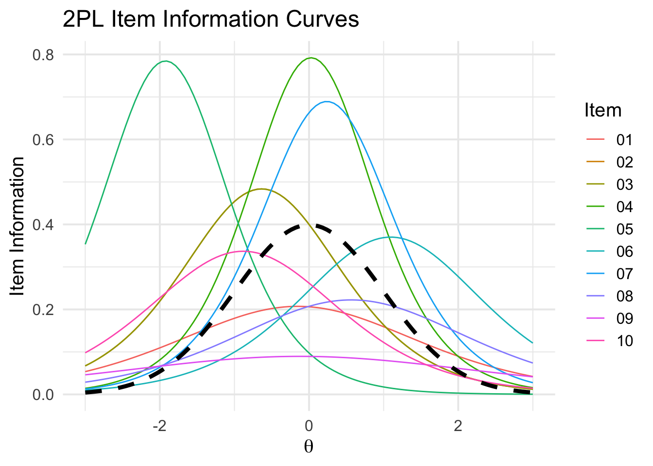
Here, the colored density lines are the item information curves for different items, and the black dotted line is the latent trait distribution (\(\theta\)) superimposed for reference. You can see that different items have higher information in different regions of the trait parameter space–some item information curves peak in the tail of \(\theta\), others more centrally, and still others show relatively flat curves across the entire latent trait distribution. These varying peaks demonstrate why different items are more-or-less informative for different people.
Why to prefer information over reliability
What do these information curves offer that \(\alpha\) does not? To see, we can first simulate responses from the 2PL IRT model given the parameters generated above, then compute \(\alpha_{\text{full}}\) on the full scale. Using \(\alpha_{\text{full}}\) as reference, we can then remove item \(i\) from the item set and calculate alpha on the resulting items (\(\alpha_{-i}\)). The difference \(\alpha_{i} = \alpha_{\text{full}} - \alpha_{-i}\) gives us an idea of how much the item \(i\) contributes to \(\alpha_{\text{full}}\). We will refer to this general method as the leave-one-item-out method. As we will cover in Part 2, the classic \(\alpha\)-based approach to item reduction would make item selections based on something akin to these \(\alpha_{i}\) values. The R code below walks through this procedure:
# simulate responses from IRT model
irt <- function(theta, a, b) {
  p <- 1 / (1 + exp(-a * (theta - b)))
  rbinom(length(p), size = 1, prob = p)
}
responses <- sapply(1:n_items, function(i) irt(theta_true, a[i], b[i]))

# two items share same characteristics + responses
# for illustration, see explanation in following text
responses[,3] <- responses[,2]

# function to calculate alpha given simulated responses
compute_alpha <- function(responses) {
  n_items <- ncol(responses)
  item_variances <- apply(responses, 2, var)
  total_variance <- var(rowSums(responses))
  (n_items / (n_items - 1)) * (1 - sum(item_variances) / total_variance)
}

# alpha on full survey
overall_alpha <- compute_alpha(responses)

# alpha minus each item
alpha_without_item <- sapply(1:n_items, function(i) {
  # Remove the i-th item from the responses matrix
  responses_without_item <- responses[, -i]
  # Calculate Cronbach's alpha for the reduced set of items
  compute_alpha(responses_without_item)
})
item_alpha_df <- data.frame(
  Item = sprintf("%02d", 1:n_items),
  alpha = alpha_without_item
)


# plot both item information and alpha with a comparison
p1 <- ggplot(item_info_long, aes(x = theta, y = Information, color = Item)) +
  geom_line() +
  labs(x = expression(theta), y = "Item information", title = "Item information curves") +
  scale_color_discrete(name = "Item") +
  theme_minimal(base_size = 15)

p2 <- ggplot(item_alpha_df, aes(x = .02*runif(10)-.01, y = overall_alpha-alpha, color = Item)) +
  geom_point(size = 4, shape = 17) +
  geom_hline(yintercept = 0, linetype=2, color = "black") +
  labs(x = "", y = expression(alpha[i]), title = "Reliability") +
  scale_x_continuous(limits = c(-0.1, 0.1)) +
  scale_color_discrete(name = "Item") +
  theme_minimal(base_size = 15) +
  theme(axis.text.x = element_blank())

(p1 + theme(legend.position = "none")) +
  p2 +
  plot_layout(widths=c(2, 1))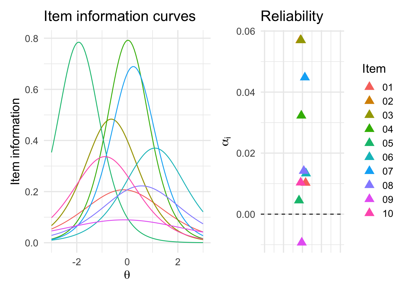
Here, we show the previous IRT-based information curves alongside the \(\alpha_{i}\) estimates from the above procedure. The higher the \(\alpha_{i}\) value, the more that the given item \(i\) contributes to \(\alpha_{\text{full}}\).
The results are rather interesting. First, we see that item 9 actually has a negative \(\alpha_{i}\) value. Indeed, \(\alpha_{\text{full}} =\) 0.708, whereas \(\alpha_{-9} =\) 0.717–reliability is actually higher in-sample without item 9. Looking at the information curves, we see that item 9 is essentially a flat curve, meaning that the item offers relatively little information across the entire trait distribution.
Second, item 5 is one of the least informative items per the \(\alpha\)-based analysis, yet we see from the information curves that item 5 is highly informative in the lower tail of \(\theta\). Therefore, removing item 5 from the scale may does not materially affect \(\alpha\), yet it will lead to a survey with a worse ability to discriminate between people with lower trait scores (i.e. lower \(\theta\)). In general, you can see by comparing the \(\alpha_{i}\) versus information curves that \(\alpha_{i}\) is generally only high when the information curve is informative near the center of the trait distribution.
Finally, items 2 and 3 both have the highest reliability contributions. If you looked through the code in detail, this may come as a surprise–we simulated items 2 and 3 as exact matches, with both the item parameters and responses all being exactly the same across respondents. Logically, given information from item 2, item 3 offers nothing new (and vice-versa), yet items 2 and 3 both have the highest rankings in terms of reliability contributions. Looking at the item curves, they don’t stick out as particularly informative. What is going on here? The answer lies in the denominator of equation (1). Recall that the variance of sum scores is made up of two parts–within item variability plus between-item covariation:
\[ \begin{equation} \text{Var}\left(\sum_{i=1}^k X_i\right) = \sum_{i=1}^k \text{Var}(X_i) + 2 \sum_{i < j} \text{Cov}(X_i, X_j) \end{equation} \] where \(\text{Cov}(X_i, X_j) = \rho_{ij} \sqrt{\text{Var}(X_i)\text{Var}(X_j)}\). With a perfect correlation (\(\rho_{2,3} = 1\)), items 2 and 3 inflate the covariance term, inflating the denominator in (1), producing higher \(\alpha\) when calculated across all 10 items. When one of the items is removed and \(\alpha\) is recalculated, the covariance term for those items drops out, and \(\alpha\) decreases in turn. This example illustrates why assumption 3 from above is so detrimental to the use of \(\alpha\)–redundant items lead to significant upward bias.
From global to local, back to global again
It is clear from the previous section that information curves offer more insight, but practically, the curves alone don’t tell us which items we should include. How do we measure the total information per a set of items, akin to what we get with \(\alpha\)? Referring back to the curves plotted above, some curves peak more centrally in the latent trait distribution (i.e. items 4 and 7), and others more in the tail (i.e. item 5). Should we just take any item with a high enough peak (high \(a\)), or should we consider where it peaks too (location of \(b\))?
Answering these questions will require us to make some assumptions about the population we are studying with our survey. Specifically, because we have a local information density as opposed to a single global value for each item, we need to integrate the information density across the assumed latent trait distribution to get the expected total information for each item:
\[ \begin{equation} \mathbb{E}[I_i] = \int I_i(\theta) p_{i}(\theta) d \theta \tag{4} \end{equation} \]
The resulting expectation \(\mathbb{E}[I_i]\) then indicates the total information for item \(i\) across the latent trait distribution. From a theoretical perspective, we should construct the latent trait distribution to best match the characteristics of the sample we aim to administer our survey to. In practice, however, we can fall back on the assumption of the underlying IRT model–in most cases, the population-level latent trait is assumed to follow a standard normal distribution (i.e. \(\theta \sim \mathcal{N}(0,1)\)).
Once the latent trait distribution is defined, we can solve (4) numerically by sampling from \(\theta\) and computing the information for each sample and item, akin to what we did above when plotting out the information curves. We can then compare the resulting expected total information values (\(\mathbb{E}[I_i]\)) to the corresponding values from the \(\alpha\)-based analysis (\(\alpha_i\)) to see how they differ:
# generate theta
theta <- rnorm(10000, 0, 1)

# compute fisher info (same a and b parameters as above)
item_fisher_info <- compute_fisher(theta, a, b)

# total info = mean across theta for each item
total_info <- apply(item_fisher_info, 2, mean)

item_info_df <- data.frame(
  Item = sprintf("%02d", 1:n_items),
  info = total_info
)

p3 <- ggplot(item_info_df, aes(x = .02*runif(10)-.01, y = info, color = Item)) +
  geom_point(size = 4, shape = 17) +
  geom_hline(yintercept = 0, linetype=2, color = "black") +
  labs(x = "", y = expression(E*"["*italic(I)[i]*"]"), title = "Fisher Information") +
  scale_x_continuous(limits = c(-0.1, 0.1)) +
  scale_color_discrete(name = "Item") +
  theme_minimal(base_size = 15) +
  theme(axis.text.x = element_blank())

(p2 + theme(legend.position = "none")) + p3
From the plot, we see that the item-level contributions are ranked similarly, but not exactly the same between the \(\alpha\)-based versus information-based item scores. Interestingly, we see that item 5 is given higher precedence by the total information metric compared to the \(\alpha\)-based metric. Additionally, redundant items 2 and 3 are not inflated as in the \(\alpha\)-based metric, although they are still ranked rather high relative to other items. In principle, if either item is in the set, we do do not need the other, so a good metric should rank them both very low. These results help solidify the story from before, but also add some nuance. Compared to \(\alpha\)-based reliability metrics, information-based metrics give us richer insights into the best items to use to measure the underlying latent trait. However, Fisher information still lacks when it comes to capturing redundancy between items.
Although we will not cover it in more depth here, it is worth noting that the total information method above allows us much more flexibility in how we want to optimize our survey. For example, if our aim was to develop a survey that was best at measuring people below the median trait value, we can take the same approach as above but just sample \(\theta < 0\) as opposed to the entire range of \(\theta\). Doing so results in item information scores that only reflect informativeness below the median trait level:
# generate theta (below 0/median only)
theta <- -abs(rnorm(10000, 0, 1))

# compute fisher info
item_fisher_info <- compute_fisher(theta, a, b)

# total info = sum across theta for each item
total_info <- apply(item_fisher_info, 2, mean)

item_info_df <- data.frame(
  Item = sprintf("%02d", 1:n_items),
  info = total_info
)

p4 <- ggplot(item_info_df, aes(x = .02*runif(10)-.01, y = info, color = Item)) +
  geom_point(size = 4, shape = 17) +
  geom_hline(yintercept = 0, linetype=2, color = "black") +
  labs(x = "", y = expression(E*"["*italic(I)[i]*"]"), title = "< 50%ile") +
  scale_x_continuous(limits = c(-0.1, 0.1)) +
  scale_color_discrete(name = "Item") +
  theme_minimal(base_size = 15) +
  theme(axis.text.x = element_blank())

(p3 + theme(legend.position = "none")) + p4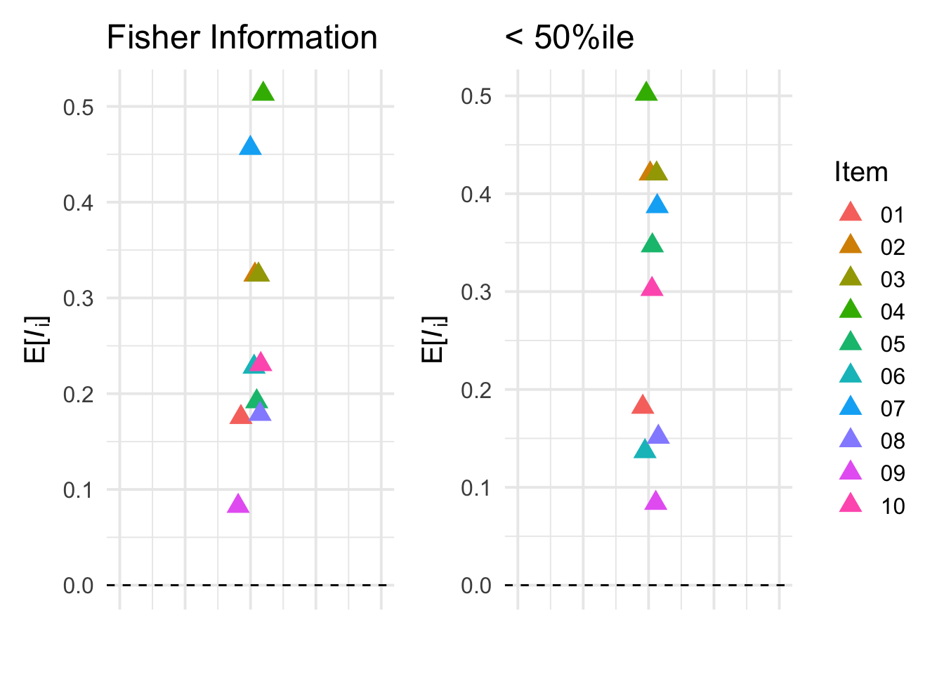
As you may expect, item 5 is even more informative relative to other items when looking only at trait levels below the median. Methods like this are particularly useful if we aim to develop a scale that will be used in settings where we need to differentiate people in particular ranges of the latent parameters space (e.g., in clinical samples where we need to differentiate between extreme levels of anxiety, depression, etc.).
Sorry Fisher, we’re going Bayesian
So far, we have made a strong case for why information-based measures are superior to \(\alpha\)-based measures when it comes to understanding how items individually contribute to latent trait measurement. However, the Fisher information measure does have some limitations. Most notably, akin to \(\alpha\), Fisher information does not account for correlation in information across items–we can see this by referring back to equations (2) and (3). There is no mechanism in the information function that could capture dependence between items. The downstream effect is that, as observed in our simulated example, items selected into a subset based solely on their total Fisher information score can lead to inclusion of redundant items.
Kullback-Leibler divergence to measure informativeness
To better account for dependence between items, we are going to expand our perspective a bit, taking inspiration from Jonas (2021). Jonas takes a Bayesian approach, where information is measured by comparing the prior versus posterior distribution on the latent trait estimate \(\theta\). Jonas uses the Kullback-Leibler divergence between the prior \(p(\theta)\) and posterior \(p(\theta | \mathbf{Y})\) as an estimate of global test information. K-L divergence is an information-theoretic measure that is defined as follows:
\[ \begin{equation} D_{\text{KL}}(P \| Q) = \int P(x) \log \frac{P(x)}{Q(x)} \, dx \tag{5} \end{equation} \] where \(P\) and \(Q\) are the distributions we are measuring distance between, and \(x\) is the underlying variable. In our case, \(P(x)\) and \(Q(x)\) refer to the prior and posterior distributions on \(\theta\), respectively, where the prior is the reference distribution. Like other distance measures, higher values indicate a greater distance. The idea here is rather intuitive then–in the absense of any information, our best guess for an person’s trait level \(\theta\) is simply the population distribution. The assumed population distribution is encoded in our prior, so a larger K-L divergence means that we have learned something about a person’s latent trait that differentiates them within the population at large.
To implement the K-L divergence method, we can first sample \(N\) trait values of \(\theta\) from the prior (\(\theta_{i} \sim \mathcal{N}(0,1)\)), generate IRT responses for each item (\(Y_{i,1:10}\)) given the sampled trait values and item parameters, and then fit the 2PL IRT model to the resulting responses. We can then compute the K-L divergence separately for each sampled trait value between the prior and the posterior that we have after fitting the model, then take the mean across trait values to get the expected K-L divergence for the set of items. We can then use the same leave-one-item-out method as for \(\alpha\) above as a measure of item informativeness:
\[ D_{\text{KL}}(P \| Q)_{i} = D_{\text{KL}}(P \| Q)_{\text{full}} - D_{\text{KL}}(P \| Q)_{-i} \]
Note that we already sampled \(\theta\) and item parameters and then simulated responses above, so we have already completed the first few steps. All that is left is to define the IRT model to fit, estimated \(\theta_i\) for each sample, and then estimate K-L divergence as described above.
First, let’s specify the Stan code 2PL IRT model:
data {
  int<lower=1> N; // Number of respondents
  int<lower=1> J; // Number of items
  array[N, J] int<lower=0, upper=1> Y; // Response matrix (N x J)
  vector<lower=0>[J] a;
  vector[J] b;
}

parameters {
  vector[N] theta; // Latent trait
}

model {
  // Priors
  theta ~ normal(0, 1);

  // Likelihood
  for (n in 1:N) {
    for (j in 1:J) {
      real eta = a[j] * (theta[n] - b[j]);
      Y[n, j] ~ bernoulli_logit(eta);
    }
  }
}
You can see that the model is quite simple–we are only actually estimating \(\theta_i\), as we are passing in the item parameters (\(a\) and \(b\)) as data given that we know the true values.
Next, we define some convenience functions that allow us to compute K-L divergence given the Stan output:
# returns the prior density at theta
prior_dens <- function(theta) {
  dnorm(theta, 0, 1)
}

# approximates posterior density given MCMC samples,
# then returns density at theta
posterior_dens <- function(post_theta, theta) {
  dens <- density(post_theta, bw = "nrd0")
  approxfun(dens$x, dens$y, rule = 2)(theta)
}

# computes K-L divergence between prior and posterior
kl_div <- function(post_theta, theta) {
  mean(
    log(
      prior_dens(theta) /
      posterior_dens(post_theta, theta)
    )
  )
}

# convenience function for extracting posterior samples
# from cmdstanr model fit
par_from_draws <- function(fit, par) {
  rvars_pars <- as_draws_rvars(
    fit$draws(
      c(par)
    )
  )
  return(lapply(rvars_pars, draws_of))
}
Finally, the function below will run the leave-one-item-out procedure and plot out the resulting \(D_{\text{KL}}(P \| Q)_{i}\) metrics:
library(foreach)
library(posterior)

estimate_info <- function(metric="kl") {
  results <- foreach(item=0:n_items, .combine = "c") %do% {
    # data without the current item
    stan_dat <- list(
      N = n_persons,
      J = n_items - if (item != 0) 1 else 0,
      Y = if (item != 0) responses[, -item] else responses,
      a = if (item != 0) a[-item] else a,
      b = if (item != 0) b[-item] else b
    )

    fit <- irt_2pl$sample(
      data = stan_dat,
      iter_sampling = 500,
      iter_warmup = 200,
      chains = 8,
      parallel_chains = 8,
      refresh = 0
    )

    # extract posteriors on theta
    post_theta <- par_from_draws(fit, "theta")$theta

    # estimate item information
    item_info <- foreach(iter=1:n_persons, .combine = "c") %do% {
      if (metric == "kl") {
        # if using K-L divergence metric
        kl_div(post_theta[,iter], seq(-4, 4, length.out = 1000))
      } else if (metric == "bf") {
        # if using bayes factor metric (hey stop reading ahead)
        bayes_factor(post_theta[,iter], theta_true[iter])
      }

    }
    # mean across theta iterations/samples to get expected info
    mean(item_info, na.rm = T)
  }
}

results <- estimate_info("kl")
item_info_df <- data.frame(
Item = sprintf("%02d", 1:n_items),
info = results[1] - results[2:11]
)
p5 <- ggplot(item_info_df, aes(x = .02*runif(10)-.01, y = info, color = Item)) +
geom_point(size = 4, shape = 17) +
geom_hline(yintercept = 0, linetype=2, color = "black") +
labs(x = "", y = expression(D[KL]("P||Q")[i]), title = "K-L Divergence") +
scale_x_continuous(limits = c(-0.1, 0.1)) +
scale_color_discrete(name = "Item") +
theme_minimal(base_size = 15) +
theme(
axis.text.x = element_blank(),
legend.position = "none"
)
(p2 + theme(legend.position = "none")) + p3 + p5 + plot_layout(nrow=2, ncol=2)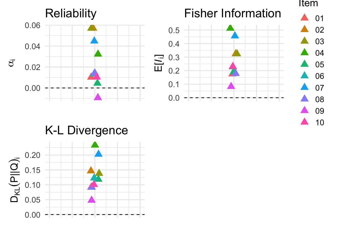
Looking at the results, the K-L divergence metric tells the same basic story as the Fisher information metric, although with a slightly higher preference for items with information curves peaking in the tail of the trait distribution (i.e. item 5).
At first, these results surprised me a bit. However, in hindsight it makes sense why we may see a pattern like this–the K-L divergence metric is largely non-specific, meaning that we can get the same K-L divergence for many potential changes in the posterior. For example, take a look at the plot below, wherein each panel has an identical K-L divergence metric despite the posterior having more uncertainty, less uncertainty, becoming bimodal, or retaining the same uncertainty but shifting over relative to the prior:
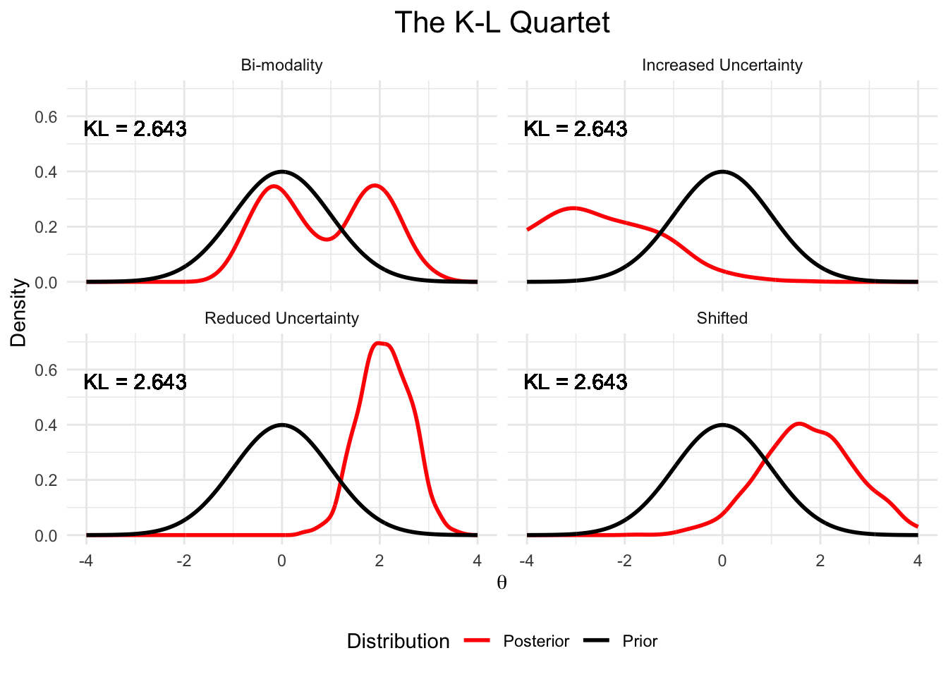
The implication for us is that K-L divergence does not indicate if our new view is any closer to the true underlying latent trait of interest. In other words, K-L divergence is agnostic to the “direction” of improvement–it evaluates the information change without accounting for whether that change aligns with the latent construct we aim to measure.
Bayes factors to measure informativeness
To resolve the non-specificity of the K-L divergence metric, but retain the idea of assessing information changes from prior to posterior, we can use Bayes factors. Unlike K-L divergence, Bayes factors can tell us the relative increase in evidence for the true latent trait value \(\theta_{i}\) from the prior to posterior.
If we have a prior distribution \(p(\theta)\) and a posterior distribution \(p(\theta | \mathbf{Y})\) for the latent trait \(\theta\) given item responses \(\mathbf{Y}\), the Bayes factor comparing the prior and posterior can be expressed as the ratio of the posterior density to the prior density evaluated at a particular value of \(\theta\), in our case the true \(\theta_i\) used to simulate the associated responses. This gives the Savage-Dickey density ratio (refer to this talk for some visuals, or Wagenmakers et al., 2010 for a write-up):
\[ BF = \frac{p(\theta = \theta_i | \mathbf{Y})}{p(\theta = \theta_i)} \]
In our context, higher values for \(BF\) would indicate that the set of items used when estimating the posterior distribution \(p(\theta | \mathbf{Y})\) is increasingly informative with respect to the true underlying trait value–this is exactly what we want!
By focusing only on evidence for the true latent trait value, in principle, the \(BF\) method should allow us to circumvent issues with both uninformative and redundant items that arose when using other item informativeness measures. To see if this actually plays out empirically, we can use the same leave-one-item-out procedure as before. We first compute the \(BF\) metric for all 10 items \(BF_{\text{full}}\), then for each item set while removing item \(i\) (\(BF_{-i}\)), and use the difference for each item (\(BF_i = BF_{\text{full}} - BF_{-i}\)) as a measure of item informativeness:
# Savage-Dickey density ratio method for (log) BF esitimate
bayes_factor <- function(post_theta, theta) {
  log(
    posterior_dens(post_theta, theta) /
    prior_dens(theta)
  )
}

results <- estimate_info("bf")
item_info_df <- data.frame(
Item = sprintf("%02d", 1:n_items),
info = results[1] - results[2:11]
)
p6 <- ggplot(item_info_df, aes(x = .02*runif(10)-.01, y = info, color = Item)) +
geom_point(size = 4, shape = 17) +
geom_hline(yintercept = 0, linetype=2, color = "black") +
labs(x = "", y = expression(BF[i]), title = "Bayes Factor") +
scale_x_continuous(limits = c(-0.1, 0.1)) +
scale_color_discrete(name = "Item") +
theme_minimal(base_size = 15) +
theme(
axis.text.x = element_blank(),
legend.position = "none"
)
(p2 + theme(legend.position = "none")) + p3 + p5 + p6 + plot_layout(nrow=2, ncol=2)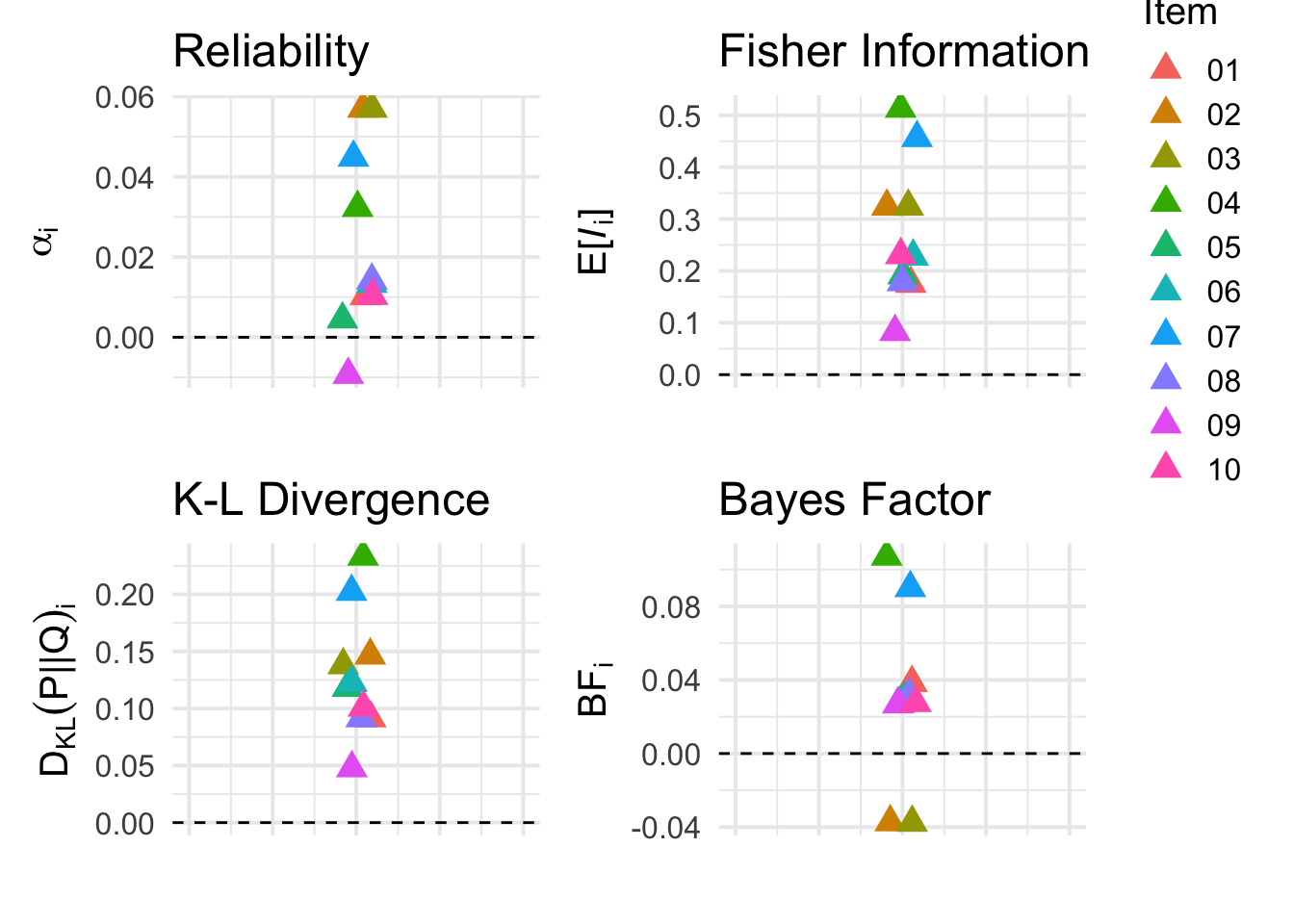
Very interesting! We see above that the \(BF_i\) metric gives a negative score to redundant items 2 and 3. This is exactly what we would expect to see if our metric is able to account for redundancy–when one of the items is in the item set, the other does not offer new information (and in fact the redundant information can actually decrease evidence for the true trait value \(\theta\)). Otherwise, the \(BF_i\) metric ranks items 4 and 7 highest, similar to other information measures. The rest of the items are all ranked rather similarly.
Part 2: Item reduction
In Part 1, we explored a wide range of different metrics that can be used to measure the informativeness of a set of survey items. We concluded with the results of the Bayes factor metric, which happened to be the only metric that was fully capable of accounting for item redundancy. In Part 2, we will turn toward actually using our various metrics to select a subset of maximally informative items from a full set–a practice typically referred to as “item reduction”.
A simple, classical approach
There are many ways that item reduction can be done, but classically, a common method was to first compute Cronbach’s \(\alpha\) (1) for a set of items, and then iteratively remove items to determine some “optimal” trade-off between survey length and reliability. We will refer to this practice as \(\alpha\)-hacking from hereon-out.
Given how easy it is to compute and interpret \(\alpha\), it makes sense why researchers have historically used \(\alpha\)-hacking to guide item reduction decisions. Of course, there is no free information lunch–\(\alpha\)-hacking can often be misleading, producing “inflated” in-sample estimates that do not generalize to out-of-sample data. More generally, in Part 1 of this post, we showed through some simulated examples how \(\alpha\) misses important information that competing measures of item informativeness readily capture. Such measures include Fisher information as well as the K-L divergence and Bayes factor measures.
A more modern, but more complicated, approach
In Part 1, we heavily relied on the leave-one-item-out procedure to test various item information metrics. Here, we will generalize the procedure, following an algorithm that relies on the same principles, but allows us to create a reduced item set of any desired size from a larger set:
- Start the “reduced item set” with 0 items,
- Fit the IRT model to the reduced set plus a new candidate item,
- Repeat step 2 for each item outside of the reduced item set,
- Once 2-3 is done for each item, identity the candidate item that is most informative and add it to the reduced item set,
- Repeat steps 2-5 until the reduced item set is of the desired length
We will call this algorithm “sequential greedy item selection”. The algorithm is considered greedy because we are taking a bit of a shortcut by not considering all the possible permutations of items that could, in theory, be better than what we arrive at by adding items to the set sequentially. However, the sequential approach is much more feasible to implement than looking at all possible subsets, especially when the candidate item set is very large. Even with just the 10 item simulated example we have been working with, it is a 10 choose K problem–if we want the best 5 items, that’s over 250 permutations! Greedy selection circumvents us needing to explore all possible permutations, at the cost of potentially not landing on the most optimal subset.
Testing out our various item reduction strategies
We are finally ready to test out our different item reduction strategies! For the K-L divergence and Bayes factor metrics, we will use the sequential greedy item selection algorithm described above. For \(\alpha\), we will take the classic approach, starting with all items and then iteratively removing items that have the least impact on \(\alpha\) until we reach the desired number of items. Finally, for the Fisher information metric, we will simply take the top \(J\) items in terms of expected item information per equation (4). We can do this for Fisher information because the information score is independent for each item, so there is no benefit to implementing a sequential search algorithm.
To determine how well the reduced sets of items perform, we will fit the 2PL IRT model to the response data for each of the reduced sets, extract the posterior estimates (\(\hat{\theta}\)), and compare them to the true values used to simulated the responses (\(\theta_i\)).
For a more realistic simulation, we will generate data for 500 people across 100 items. For each metric, we will use the corresponding item reduction method to create a reduced set of just 20 items from the 100 item full set.
To start, we will specify the sequential greedy item selection algorithm:
library(foreach)
library(posterior)

# sequential greedy item reduction algorithm using KL or BF
reduce_items <- function(desired_length, metric, responses, theta_true) {
  reduced_item_set <- c()

  while (length(reduced_item_set) < desired_length) {
    # item_set stores the information score for each item
    item_set <- foreach(item=1:ncol(responses), .combine = "c") %do% {
      if (!(item %in% reduced_item_set)) {
        # item = the current candidate item
        which_items <- c(reduced_item_set, item)

        # include only the current reduced item set + candidate item
        stan_dat <- list(
          N = n_persons,
          J = length(which_items),
          Y = as.matrix(responses[,which_items]),
          a = a[which_items],
          b = b[which_items]
        )

        fit <- irt_2pl$sample(
          data = stan_dat,
          iter_sampling = 200,
          iter_warmup = 100,
          chains = 8,
          parallel_chains = 8,
          refresh = 0
        )

        # extract posteriors on theta
        post_theta <- par_from_draws(fit, "theta")$theta

        # estimate item information
        item_info <- foreach(iter=1:n_persons, .combine = "c") %do% {
          if (metric == "kl") {
            # if using K-L divergence metric
            kl_div(post_theta[,iter], seq(-4, 4, length.out = 1000))
          } else if (metric == "bf") {
            # if using bayes factor metric
            bayes_factor(post_theta[,iter], theta_true[iter])
          }
        }
        # mean across theta iterations/samples to get expected info
        item_info <- mean(item_info, na.rm = T)
      } else {
        item_info <- -Inf
      }
      rm(fit); gc()
      return(item_info)
    }
    # add the candidate item that adds most info to the reduced set
    reduced_item_set <- c(reduced_item_set, which.max(item_set))
  }
  return(reduced_item_set)
}
Next, we will define the iterative \(\alpha\) method. To do so, we will leverage the psych package, a popular psychometrics library that researchers use in practice when performing these types of analyses:
library(psych)

# iteratively remove "worse" items per alpha
reduce_items_alpha <- function(desired_length, responses) {
  colnames(responses) <- 1:ncol(responses)
  selected_items <- colnames(responses)

  while (length(selected_items) > desired_length) {
    alpha_result <- alpha(responses[, selected_items, drop = FALSE])
    # Find the item whose removal produces highest alpha
    rm_idx <- which.max(alpha_result$alpha.drop$raw_alpha)
    item_to_remove <- rownames(alpha_result$alpha.drop[rm_idx,])
    selected_items <- setdiff(selected_items, item_to_remove)
  }
  return(as.numeric(selected_items))
}
Lastly, the Fisher information method can be specified rather easily as follows:
reduce_items_fisher <- function(desired_length, a, b) {
  # sample from the prior
  theta <- rnorm(10000)

  # compute fisher info for each item, take expectation
  # for expected fisher info
  fisher_info <- compute_fisher(theta, a, b)
  expected_info <- apply(fisher_info, 2, mean)

  # take top J items ranked by expected info
  selected_items <- order(expected_info, decreasing = TRUE)[1:desired_length]

  return(selected_items)
}
Time to simulate data and test our strategies! Note that this code chunk takes a long time to run, so consider yourself warned if you are planning to run it:
set.seed(123)

# how many items to keep
n_keep <- 15

# simulate data
n_persons <- 500
n_items <- 100
theta_true <- rnorm(n_persons)

# simulate item parameters
a <- runif(n_items, 0.5, 2)
b <- runif(n_items, -2, 2)

# simulate responses
responses <- sapply(1:n_items, function(i) irt(theta_true, a[i], b[i]))

# add in some problematic redundancy for good measure (:<
redundant_items <- sample(2:100, 30)
a[redundant_items-1] <- a[redundant_items]
b[redundant_items-1] <- b[redundant_items]
responses[,redundant_items-1] <- responses[,redundant_items]

# K-L divergence method (warning: takes a while to run!)
reduced_set_kl <- reduce_items(n_keep, "kl", responses, theta_true)

# BF method (warning: takes a while to run!)
reduced_set_bf <- reduce_items(n_keep, "bf", responses, theta_true)

# alpha method
reduced_set_alpha <- reduce_items_alpha(n_keep, responses)

# Fisher info method
reduced_set_fisher <- reduce_items_fisher(n_keep, a, b)
… one day later …
Alright! Finally done… First, let’s take a look at the reduced item sets that are different methods landed on:
| KL | BF | alpha | Fisher |
|---|---|---|---|
| 72 | 73 | 13 | 72 |
| 73 | 61 | 14 | 73 |
| 48 | 72 | 16 | 52 |
| 52 | 48 | 17 | 48 |
| 70 | 52 | 41 | 70 |
| 89 | 76 | 42 | 71 |
| 34 | 96 | 52 | 41 |
| 97 | 41 | 54 | 42 |
| 69 | 89 | 55 | 89 |
| 3 | 19 | 61 | 61 |
| 61 | 21 | 70 | 3 |
| 42 | 85 | 71 | 76 |
| 22 | 3 | 72 | 69 |
| 14 | 24 | 73 | 54 |
| 5 | 66 | 76 | 55 |
For all but the \(\alpha\) items, the ordering above roughly translates to how informative each item is as determined per the associated item reduction method. Overall, we do see overlap in which items are selected across metrics, with the most overlap between the Fisher information and K-L divergence metrics. In hindsight, this should not be too surprising given that these metrics capture information in similar ways. The \(\alpha\) metric gives quite a different set of items compared to other metrics, whereas the \(BF\) metric shows some overlap with other information-theoretic metrics but not so much with \(\alpha\).
To see which set actually performs best in terms of recovering the true underlying \(\theta\) values used to simulate responses, we fit the 2PL IRT model to each reduced set below and save out the posterior means (\(\hat{\theta}\)):
reduced_sets <- list(
  `3 K-L Divergence` = reduced_set_kl,
  `4 Bayes Factor` = reduced_set_bf,
  `1 Cronbach's alpha` = reduced_set_alpha,
  `2 Fisher Information` = reduced_set_fisher
)

post_theta_means <- foreach(set=names(reduced_sets), .combine = "rbind") %do% {
  items <- reduced_sets[[set]]
  stan_dat <- list(
    N = n_persons,
    J = length(items),
    Y = responses[,items],
    a = a[items],
    b = b[items]
  )
  fit <- irt_2pl$sample(
    data = stan_dat,
    iter_sampling = 500,
    iter_warmup = 200,
    chains = 8,
    parallel_chains = 8,
    refresh = 0
  )
  post_theta <- par_from_draws(fit, "theta")$theta

  data.frame(
    metric = set,
    person = 1:n_persons,
    theta_true = theta_true,
    theta_est = apply(post_theta, 2, mean)
  )
}
Finally, let’s take a look at the results we have been working toward! Below, we plot out the true versus estimated \(\theta\) values for each metric:
library(dplyr)

# show r2 in plot
r2s <- post_theta_means %>%
  group_by(metric) %>%
  summarize(r2 = round(cor(theta_true, theta_est)^2, 2), .groups = "drop")

ggplot(post_theta_means, aes(x = theta_true, y = theta_est)) +
  geom_point(color = "gray") +
  geom_abline(intercept = 0, slope = 1, linetype=2) +
  facet_wrap("metric", ncol=2) +
  xlab(expression(theta[true])) +
  ylab(expression(hat(theta))) +
  geom_text(
    data = r2s,
    aes(x = -2, y = 2,
        label = paste0("r2 = ", r2)),
        inherit.aes = FALSE
  ) +
theme_minimal(base_size = 15) 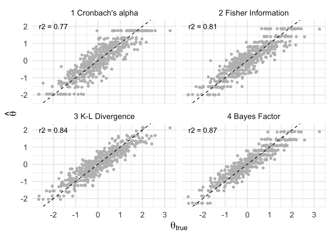
Above, the \(r^2\) value is shown on each panel for interpretability. We see that the Bayes factor method produces \(\hat{\theta}\)s that best align with the true values, followed closely by the K-L divergence and Fisher information metrics. The \(\alpha\)-hacking method then performs the worse overall, which we may expect given the item redundancy we baked into the simulated data.
Overall, I’d say these results are pretty good considering we reduced the original item pool from 100 to just 15 items–an 85% reduction!
Discussion
In this post, we explored various methods for ascertaining the information contained in survey items. In Part 1, we learned how all of Cronbach’s \(\alpha\), Fisher information, K-L divergence, and Bayes factors could be used to measure item informativeness. We also learned about some downsides of different metrics. For example, we illustrated that \(\alpha\) and Fisher information do a particularly poor job accounting for item redundancy. Additionally, we found that K-L divergence is a good measure of overall item informativeness, but that it does not tell us if the direction of information change is “correct” in the sense that it reliably captures the desired underlying latent trait. Part 1 then wrapped up with an overview of how Bayes factors can account for the shortcomings of K-L divergence.
In Part 2, we then demonstrated how our various metrics could be used to implement item reduction in practice, and we compared performance across methods. We found that the Bayes factor method performed best, followed by K-L divergence, Fisher information, and then \(\alpha\) methods. In fact, the Bayes factor method accounted for 10% more variance in the true \(\theta\) values compared to the \(\alpha\)-hacking method–a rather large difference! Although the Bayes factor method is quite computationally intensive, such a large increase in measurement precision is often worthwhile, especially when we consider that this procedure only needs to be run once.
Future directions
We only explored item reduction strategies here with a relatively simple 2PL IRT model. In the future, I believe researchers would benefit from comparing the Bayes factor and K-L divergence metrics (using the sequential greedy item selection algorithm) to competing methods on a wider variety of IRT models. In my own industry work, I have used the Bayes factor method to great success when reducing down an 11 factor, 224 item survey to just 30 items. In that application, I used a multidimensional graded response model as opposed to something simple such as the 2PL IRT model we used throughout this post.
Additionally, we have focused here wholly on item selection for item reduction purposes, but there is an entire body of research on computerized adaptive testing that our methods could be applied to. The idea here is that, instead of performing item reduction up front to create the same survey for every respondent, we can instead determine the optimal item one-by-one–with each new response, we learn more about the person’s latent trait, and as a result we can select new items that help us best estimate the respondent’s trait level given our current state of knowledge. Indeed, Bayesian methods are very popular for such adaptive design optimization tasks. There are now even some open-source packages that help users implement Bayesian adaptive design optimization in the context of behavioral tasks. Using such methods to enhance survey informativeness and efficiency in a more widespread way could really impact the way we conduct research throughout the social and behavioral sciences.
That is all for now! I hope you enjoyed the post, feel free to comment or reach out with any questions (or errata.. ) :D
Nathaniel Haines
Senior Manager, Data Science
An academic Bayesian who is currently exploring the high dimensional posterior distribution of life